
As a kid, I was obsessed with maps. Give me an atlas and I would be sucked in for hours. Eventually I wound up in coastal engineering and took a GIS course with the amazing Dr. Kate Parks in Southampton. This reignited my interest in cartography, as I now had the tools I needed to make my own maps. Over the coming years this led to an interest in how we can map our coastal regions to better communicate their morphodynamics. Also (mostly), I just wanted to make pretty maps! Making figures sometimes feels like one of the only avenues for artistic expression that we have in science.
To reach these goals, a good colourmap is a key ingredient. For a map showing the topography/bathymetry of a coast, a colourmap is the range of colours that correspond to a particular elevation. In this post, I will walk you through how I created two of my favourite colourmaps.
Example: SEAWAD Colourmap
My PhD research focused on understanding the sediment dynamics of ebb-tidal deltas, which are basically giant piles of sand that sit at the mouth of tidal inlets between barrier islands. In developing this colourmap, I was particularly interested in highlighting the shoals and channels that are moving around. Ultimately we used this colourmap in most of my PhD research and parts of the SEAWAD project.

I literally spent a week fine-tuning this colourmap, so I was initially quite protective of my work. Over the years I have had several people ask me how I made it, but I was reluctant to share my code (even though it would have been easy to reverse-engineer it if one were so inclined). However, over the past few years I realized that science doesn’t go anywhere if you keep it all to yourself, so in the interests of openness, you can find my MATLAB code here:
function [cmap] = seawadColormap
    %% seawadColormap.m Stuart Pearson's fun bathymetry colourmap
    % (c) Stuart G. Pearson, 2022. (CC BY 4.0)
    %   The fun colourmap I used for the SEAWAD bathymetric maps

    dz=0.1; % vertical spacing [m]

    % colours in colormap
    baseColours = ...
        [0 67 143;... % dark blue: -20 m NAP
        13 182 255;... % light blue: -10 m NAP
        255 255 255;... % white: -5 m NAP
        199 181 181;... % light brown: -2 m NAP
        158 144 144;... % muddy brown: 2 m NAP
        29 89 74;... % dark green: 10 m NAP
        29 89 74]./255; % dark green: 10 m NAP

    % intervals at which colour changes
    vertSpacing = [-20; -10; -5; -2; 2; 3; 10];

    % loop through and create new colourmap
    cc=1;
    for ii = 1:length(baseColours)-1
        for jj = 1:floor((vertSpacing(ii+1)-vertSpacing(ii))./dz)
            for kk = 1:3
                cmap(cc,kk) = interp1([vertSpacing(ii) vertSpacing(ii+1)],...
                    [baseColours(ii,kk) baseColours(ii+1,kk)],...
                    vertSpacing(ii)+jj.*dz);
            end
            cc=cc+1;
        end
    end
end
The choice of colours here was largely just a matter of playing around until I found shades that I liked. I love that shade of blue, and wanted to have a muddy sort of brown for the intertidal zone similar to what you can see in aerial photos of the site. Higher elevations are a dark green to match the lush vegetation that grows here in the Netherlands. You can change the colours to match your own site by changing the RGB values (0-255) in baseColours.
A key consideration when making colourmaps is to make sure that they are visible even to readers with colour vision deficiencies or when printing in black and white. In these cases, a single gradient from dark to light is often ideal, but there are many different approaches to designing accessible colourmaps (see here or the fantastic ColorBrewer, for instance). Unfortunately my SEAWAD colourmap does not quite pass muster on this front, but for most of my non-cartographic work I prefer to use the parula colourmap, which is a bit friendlier.
To adjust the smoothness of the colour transitions, set the dz value. Right now it is set at 0.1 m, which yields a pretty smooth gradient. Setting it to larger values makes the transitions look a bit more abrupt. To change the elevations at which the colours transition, change the values in vertSpacing. These values were chosen to highlight the shoals I was most interested in for my research, and also to denote intertidal areas more clearly. The deepest parts of Ameland Inlet are 25-30 m deep, but all of the interesting stuff happens above the 20 m depth contour, so I focused the colour map on higher values. In the map above, I have plotted lines at mean low water and -6 m to make these transitions more clear. However, depending on the characteristics of your site, you may want to adjust these values. Be careful about the choices you make — by focusing on a specific range of values like this, you run the risk of missing out on relevant behaviour happening at other depths!
The output variable cmap is a 3 x n array that you can feed into the colormap function in MATLAB, just as you would with another colormap like parula or jet.
If you use this colourmap or code, I would appreciate some credit/an acknowledgement (as per CC BY 4.0). Most of all I would love to hear from you and see your maps!
Example: Vintage Colourmap
In the past few years, I have spent a lot of time and energy poring over old maps of Ameland with my colleague Edwin Elias. In our 2019 paper, we used these maps to better understand how the ebb-tidal delta has evolved through time:
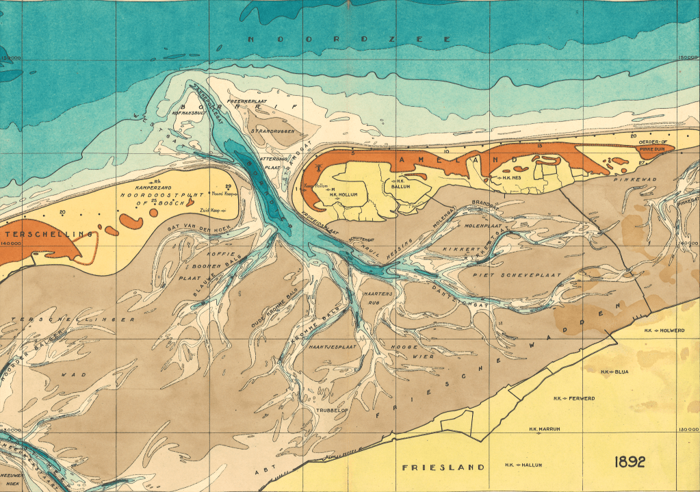
While these maps have great scientific value, they are also just gorgeous. Originally prepared as nautical charts by the Hydrographic Service of the Royal Netherlands Navy, these maps have a very cool vintage look, which I wanted to replicate for my own figures.
To do this, I used the eyedropper tool in Adobe Illustrator to identify the shades used to represent each elevation on the map (baseColours). With a bit of guesswork, I then tried to assign similar elevations in vertSpacing, which in this version of the function I pass in as an external variable. Beyond that, it is much the same as the SEAWAD colourmap function above. Using similar principles, you can create your own custom colourmaps too!
function [cmap] = vintageColormap(vertSpacing)
    %% vintageColormap.m
    % (c) Stuart G. Pearson, 2022.  (CC BY 4.0)
    % Vintage bathymetry colourmap from Edwin/Albert's old 1950s Wadden Sea Maps
    % See Elias et al 2019
    % takes in vertSpacing, a 10-column array with elevations of each contour

    % intervals at which colour changes:
    %    vertSpacing = [-20; -16; -12; -8; -5; -3; -1.2; 0; 1.4; 10];

    dz=0.1; % vertical spacing

    % colours in colormap
    baseColours = ...
        [27 126 129;... % Deepest (darkest green-blue): -20 m NAP
        41 155 151;... % Deeper (dark green-blue): -16 m NAP
        56 170 164;... % Deep (green-blue): -12 m NAP
        130 199 180;... % Subtidal (light green-blue): -8 m NAP
        220 231 194;... % Shallow Subtidal (lighter green blue): -5 m NAP
        255 240 196;... % Shoal (off-white): -3 m NAP
        244 214 176;... % Low Tide (light brown): -1.2 m NAP
        217 188 146;... % High Tide (darker brown): 0 m NAP
        255 221 146;... % Beach (yellowy brown): 1.4 m NAP
        226 129 61]./255; % Dune (orange): 10 m NAP

    % loop through and create new colourmap
    cc=1;
    for ii = 1:length(baseColours)-1
        for jj = 1:floor((vertSpacing(ii+1)-vertSpacing(ii))./dz)
            for kk = 1:3
                cmap(cc,kk) = interp1([vertSpacing(ii) vertSpacing(ii+1)],...
                    [baseColours(ii,kk) baseColours(ii+1,kk)],...
                    vertSpacing(ii)+jj.*dz);
            end
            cc=cc+1;
        end
    end

end
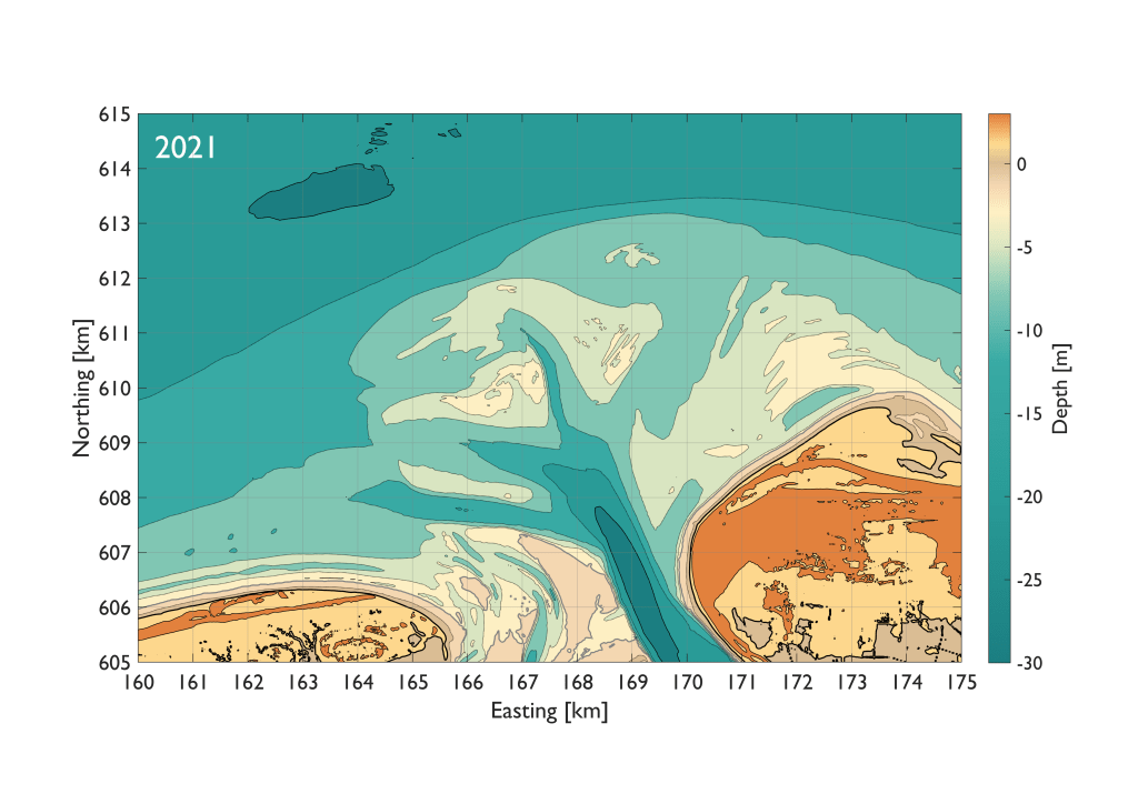
Here we can see the results, with modern bathymetry from 2021 (the same dataset as in the SEAWAD figure earlier on). This colourmap puts a bit less focus on the ebb-tidal shoals, but we could adjust that by changing vertSpacing.
Hopefully this is interesting and/or useful to somebody out there. As I mentioned above, I would appreciate an acknowledgement if you use this in your research (as per CC BY 4.0). Most of all, I would love to hear from you and see your maps!
Sources:
Elias, E. P., Van der Spek, A. J., Pearson, S. G., & Cleveringa, J. (2019). Understanding sediment bypassing processes through analysis of high-frequency observations of Ameland Inlet, the Netherlands. Marine Geology, 415, 105956.
